Shortcut Layer

Deep Neural Networks model suffer from the degradation problem, i.e. the accuracy reduction with increasing depth of the network; Moreover, the accuracy loss happens in the training dataset.

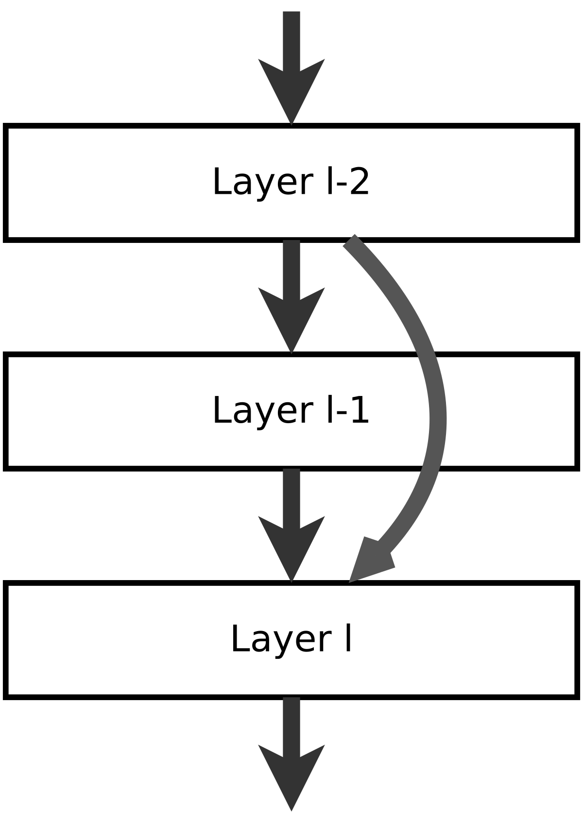
In the original paper, they addres the degradation problem by introducing a deep residual learning framework, or shortcut connections, that skips one ore more layers (as shown in the figure below), without introducing extra parameters or computational cost.

In the original paper, the shortcut connections perform an operation like:

Where F(x) is the ouput of layer l-1, x is the output of the layer l-2, and H(x) is the output of the layer l, or Shortcut_layer (see image below for reference).

The object Shortcut_layer is an implementation of this concept, where is possible to add weights to the linear combination, α and β, as :

And it can actually deal with different sized inputs. The code below shows an example on how to use the single shortcut layer forward and backward:

# first the essential import for the library.
# after the installation:
from NumPyNet.layers.shortcut_layer import Shortcut_layer # class import
from NumPyNet import activations

import numpy as np # the library is entirely based on numpy

# define a batch of images (even a single image is ok, but is important that it has all the four dimensions) in the format (batch, width, height, channels)

batch, w, h, c = (5, 100, 100, 3) # batch != 1 in this case
input1 = np.random.uniform(low=0., high=1., size=(batch, w, h, c)) # you can also import some images from file
input2 = np.random.uniform(low=0., high=1., size=(batch, w, h, c)) # second input

alpha = 0.75
beta  = 0.5

activ_func = activations.Relu() # it can also be:
															 #     activations.Relu  (class Relu)
															 #     "Relu" (a string, case insensitive)

# Layer initialization, with parameters scales and bias
layer = Shortcut_layer(activation=activ_func, alpha=0.75, beta=0.5)


# Forward pass
layer.forward(inpt=input1, prev_output=input2)
out_img = layer.output    # the output in this case will be a batch of images of shape = (batch, out_width, out_heigth , out_channels)

# Backward pass
delta       = np.random.uniform(low=0., high=1., size=input.shape)     # definition of network delta, to be backpropagated
layer.delta = np.random.uniform(low=0., high=1., size=out_img.shape)   # layer delta, ideally coming from the next layer
layer.backward(delta, copy=False)

# now net_delta is modified and ready to be passed to the previous layer.delta
# and also the updates for weights and bias are computed in the backward

To have a look more in details on what’s happening, the defintions of forward and backward are:

def forward(self, inpt, prev_output):
	'''
	Forward function of the Shortcut layer: activation of the linear combination between input

	Parameters:
		inpt        : array of shape (batch, w, h, c), first input of the layer
		prev_output : array of shape (batch, w, h, c), second input of the layer
	'''
	# assert inpt.shape == prev_output.shape

	self._out_shape = [inpt.shape, prev_output.shape]

	if inpt.shape == prev_output.shape:
		self.output = self.alpha * inpt[:] + self.beta * prev_output[:]

	else:

		# If the layer are combined the smaller one is distributed according to the
		# sample stride
		# Example:
		#
		# inpt = [[1, 1, 1, 1],        prev_output = [[1, 1],
		#         [1, 1, 1, 1],                       [1, 1]]
		#         [1, 1, 1, 1],
		#         [1, 1, 1, 1]]
		#
		# output = [[2, 1, 2, 1],
		#           [1, 1, 1, 1],
		#           [2, 1, 2, 1],
		#           [1, 1, 1, 1]]

		if (self.ix, self.iy, self.kx) is (None, None, None):
			self._stride_index(inpt.shape, prev_output.shape)

		self.output = inpt.copy()
		self.output[:, ix, jx, kx] = self.alpha * self.outpu[:, ix, jx, kx] + self.beta * prev_output[:, iy, jy, ky]


	self.output = self.activation(self.output)
	self.delta = np.zeros(shape=self.out_shape, dtype=float)

If the shapes of the two inputs are identical, then the output is the simple linear combinations of the two. If that’s not the case, the function _stride_index computes the indices (for both inputs) which corresponding positions will be combined togheter.

def backward(self, delta, prev_delta):
	'''
	Backward function of the Shortcut layer

	Parameters:
		delta      : array of shape (batch, w, h, c), first delta to be backpropagated
		delta_prev : array of shape (batch, w, h, c), second delta to be backporpagated

	'''

	# derivatives of the activation funtion w.r.t. to input
	self.delta *= self.gradient(self.output)

	delta[:]   += self.delta * self.alpha

	if (self.ix, self.iy, self.kx) is (None, None, None): # same shapes
		prev_delta[:] += self.delta[:] * self.beta

	else: # different shapes
		prev_delta[:, self.ix, self.jx, self.kx] += self.beta * self.delta[:, self.iy, self.jy, self.ky]

backward makes use of the same indixes to backpropagate delta for both input layers.